 View on QuantumAI View on QuantumAI
|
 Run in Google Colab Run in Google Colab
|
 View source on GitHub View source on GitHub
|
|
In this tutorial, we implement the quantum approximate optimization algorithm (QAOA) for determining the Max-Cut of the Sycamore processor's hardware graph (with random edge weights). Max-Cut is the NP-complete problem of finding a partition of the graph's vertices into an two distinct sets that maximizes the number of edges between the two sets. To do so, we will:
- Define a random set of weights over the hardware graph.
- Construct a QAOA circuit using Cirq.
- Calculate the expected value of the QAOA cost function.
- Create an outer loop optimization to minimize the cost function.
- Compare cuts found from QAOA with random cuts.
try:
    import cirq
except ImportError:
    print("installing cirq...")
    !pip install --quiet cirq
    import cirq

    print("installed cirq.")
1. Defining a random set of weights over the hardware graph
In order to make the problem easily embeddable on a quantum device, we will look at the problem of Max-Cut on the same graph that the device's qubit connectivity defines, but with random valued edge weights.
from typing import List
import sympy
import numpy as np
import matplotlib.pyplot as plt

import cirq_google

working_device = cirq_google.Sycamore
print(working_device)
(0, 5)───(0, 6)
                                             │        │
                                             │        │
                                    (1, 4)───(1, 5)───(1, 6)───(1, 7)
                                    │        │        │        │
                                    │        │        │        │
                           (2, 3)───(2, 4)───(2, 5)───(2, 6)───(2, 7)───(2, 8)
                           │        │        │        │        │        │
                           │        │        │        │        │        │
                  (3, 2)───(3, 3)───(3, 4)───(3, 5)───(3, 6)───(3, 7)───(3, 8)───(3, 9)
                  │        │        │        │        │        │        │        │
                  │        │        │        │        │        │        │        │
         (4, 1)───(4, 2)───(4, 3)───(4, 4)───(4, 5)───(4, 6)───(4, 7)───(4, 8)───(4, 9)
         │        │        │        │        │        │        │        │
         │        │        │        │        │        │        │        │
(5, 0)───(5, 1)───(5, 2)───(5, 3)───(5, 4)───(5, 5)───(5, 6)───(5, 7)───(5, 8)
         │        │        │        │        │        │        │
         │        │        │        │        │        │        │
         (6, 1)───(6, 2)───(6, 3)───(6, 4)───(6, 5)───(6, 6)───(6, 7)
                  │        │        │        │        │
                  │        │        │        │        │
                  (7, 2)───(7, 3)───(7, 4)───(7, 5)───(7, 6)
                           │        │        │
                           │        │        │
                           (8, 3)───(8, 4)───(8, 5)
                                    │
                                    │
                                    (9, 4)
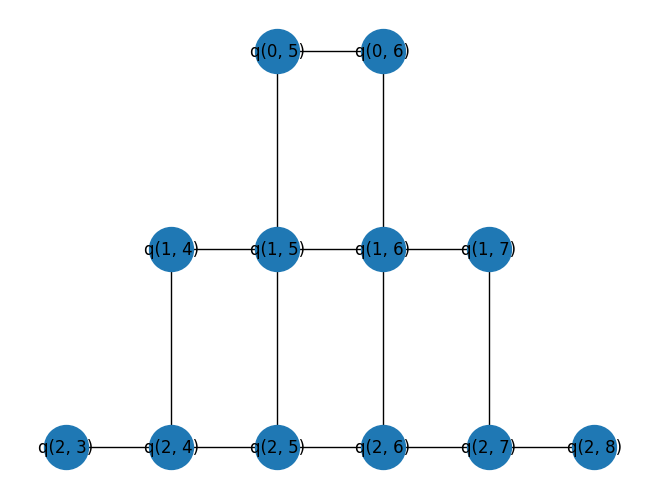
Since a circuit covering the entire Sycamore device cannot be easily simulated, a small subset of the device graph will be used instead.
import networkx as nx

# Set the seed to determine the problem instance.
np.random.seed(seed=11)

# Identify working qubits from the device.
device_qubits = working_device.metadata.qubit_set
working_qubits = sorted(device_qubits)[:12]

# Populate a networkx graph with working_qubits as nodes.
working_graph = working_device.metadata.nx_graph.subgraph(working_qubits)

# Add random weights to edges of the graph. Each weight is a 2 decimal floating point between 0 and 5.
nx.set_edge_attributes(
    working_graph,
    {e: {"weight": np.random.randint(0, 500) / 100} for e in working_graph.edges},
)

# Draw the working_graph on a 2d grid
pos = {q: (q.col, -q.row) for q in working_graph.nodes()}
nx.draw(working_graph, pos=pos, with_labels=True, node_size=1000)
plt.show()
2. Construct the QAOA circuit
Now that we have created a Max-Cut problem graph, it's time to generate the QAOA circuit following Farhi et al.. For simplicity, \(p = 1\) is chosen.
from cirq.contrib.svg import SVGCircuit

# Symbols for the rotation angles in the QAOA circuit.
alpha = sympy.Symbol("alpha")
beta = sympy.Symbol("beta")

qaoa_circuit = cirq.Circuit(
    # Prepare uniform superposition on working_qubits == working_graph.nodes
    cirq.H.on_each(working_graph.nodes()),
    # Do ZZ operations between neighbors u, v in the graph. Here, u is a qubit,
    # v is its neighboring qubit, and w is the weight between these qubits.
    (
        cirq.ZZ(u, v) ** (alpha * w["weight"])
        for (u, v, w) in working_graph.edges(data=True)
    ),
    # Apply X operations along all nodes of the graph. Again working_graph's
    # nodes are the working_qubits. Note here we use a moment
    # which will force all of the gates into the same line.
    cirq.Moment(cirq.X(qubit) ** beta for qubit in working_graph.nodes()),
    # All relevant things can be computed in the computational basis.
    (cirq.measure(qubit) for qubit in working_graph.nodes()),
)
SVGCircuit(qaoa_circuit)
3. Calculating the expected value of the QAOA cost Hamiltonian
Now that we have created a parameterized QAOA circuit, we need a way to calculate expectation values of the cost Hamiltonian. For Max-Cut, the cost Hamiltonian is
\[ H_C = \frac{1}{2} \sum_{\langle i, j\rangle} w_{ij} (1 - Z_i Z_j ) \]
where \(\langle i, j \rangle\) denotes neighboring qubits, \(w_{ij}\) is the weight of edge \(ij\), and \(Z\) is the usual Pauli-\(Z\) matrix. The expectation value of this cost Hamiltonian is \(\langle \alpha, \beta | H_C | \alpha, \beta \rangle\) where \(|\alpha, \beta\rangle\) is the quantum state prepared by our qaoa_circuit. This is the cost function we need to estimate.
Pauli-\(Z\) has eigenvalues \(\pm 1\). If qubits \(i\) and \(j\) are in the same eigenspace, then \(\langle Z_i Z_j \rangle = 1\) and so \(\frac{1}{2} w_{ij} \langle 1 - Z_i Z_j \rangle = 0\). In the Max-Cut language, this means that edge \(ij\) does not contribute to the cost. If qubits \(i\) and \(j\) are in the opposite eigenspace, then \(\langle Z_i Z_j \rangle = -1\) and so \(\frac{1}{2} w_{ij} \langle 1 - Z_i Z_j \rangle = w_{ij}\). In the Max-Cut language, this means that edge \(ij\) contributes its weight \(w_{ij}\) to the cost.
To estimate the cost function, we need to estimate the (weighted) sum of all \(ZZ\) pairs in the graph. Since these terms are diagonal in the same basis (namely, the computational basis), they can measured simultaneously. Given a set of measurements (samples), the function below estimates the cost function.
import pandas as pd


def estimate_cost(graph: nx.Graph, samples: pd.DataFrame) -> float:
    """Estimate the cost function of the QAOA on the given graph using the
    provided computational basis bitstrings."""
    cost_value = 0.0

    # Loop over edge pairs and compute contribution.
    for u, v, w in graph.edges(data=True):
        u_samples = samples[str(u)]
        v_samples = samples[str(v)]

        # Determine if it was a +1 or -1 eigenvalue.
        u_signs = (-1) ** u_samples
        v_signs = (-1) ** v_samples
        term_signs = u_signs * v_signs

        # Add scaled term to total cost.
        term_val = np.mean(term_signs) * w["weight"]
        cost_value += term_val

    return -cost_value
Now we can sample from the qaoa_circuit and use estimate_expectation to calculate the expectation value of the cost function for the circuit. Below, we use arbitrary values for \(\alpha\) and \(\beta\).
alpha_value = np.pi / 4
beta_value = np.pi / 2
sim = cirq.Simulator()

sample_results = sim.sample(
    qaoa_circuit, params={alpha: alpha_value, beta: beta_value}, repetitions=20_000
)
print(f"Alpha = {round(alpha_value, 3)} Beta = {round(beta_value, 3)}")
print(f"Estimated cost: {estimate_cost(working_graph, sample_results)}")
Alpha = 0.785 Beta = 1.571
Estimated cost: -0.728132
4. Outer loop optimization
Now that we can compute the cost function, we want to find the optimal cost. There are lots of different techniques to choose optimal parameters for the qaoa_circuit. Since there are only two parameters here (\(\alpha\) and \(\beta\)), we can keep things simple and sweep over incremental pairings using np.linspace and track the minimum value found along the way.
# Set the grid size = number of points in the interval [0, 2π).
grid_size = 5

alpha_sweep = cirq.Linspace(alpha, 0, 2 * np.pi, grid_size)
beta_sweep = cirq.Linspace(beta, 0, 2 * np.pi, grid_size)
samples = sim.run_sweep(
    qaoa_circuit, params=alpha_sweep * beta_sweep, repetitions=20000
)

exp_values = np.reshape(samples, (-1, grid_size)).tolist()
estimate = np.vectorize(lambda s: estimate_cost(working_graph, s.data))
exp_values = estimate(exp_values)
par_tuples = [tuple(y[1] for y in x) for x in (alpha_sweep * beta_sweep).param_tuples()]
par_values = np.reshape(par_tuples, (-1, grid_size, 2))
We can now visualize the cost as a function of \(\alpha\) and \(\beta\).
plt.title("Heatmap of QAOA Cost Function Value")
plt.xlabel(r"$\alpha$")
plt.ylabel(r"$\beta$")
plt.imshow(exp_values)
plt.show()
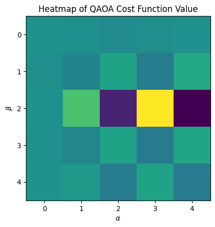
This heatmap is coarse because we selected a small grid_size. To see more detail in the heatmap, one can increase the grid_size.
5. Compare cuts
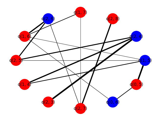
We now compare the optimal cut found by QAOA to a randomly selected cut. The helper function draws the working_graph and colors nodes in different sets different colors. Additionally, we print out the cost function for the given cut.
def output_cut(s_partition: List[cirq.Qid]) -> None:
    """Plot and output the graph cut information."""

    # Generate the colors.
    coloring = []
    for node in working_graph:
        if node in s_partition:
            coloring.append("blue")
        else:
            coloring.append("red")

    # Get the weights
    edges = working_graph.edges(data=True)
    weights = [w["weight"] for (u, v, w) in edges]

    nx.draw_circular(
        working_graph,
        node_color=coloring,
        node_size=1000,
        with_labels=True,
        width=weights,
    )
    plt.show()
    size = nx.cut_size(working_graph, s_partition, weight="weight")
    print(f"Cut size: {size}")
As an example, we can test this function with all nodes in the same set, for which the cut size should be zero.
# Test with the empty S and all nodes placed in T.
output_cut([])
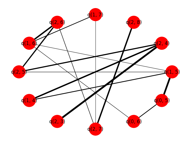
Cut size: 0
To get cuts using the QAOA we will first need to extract the best control parameters found during the sweep:
best_exp_index = np.unravel_index(np.argmax(exp_values), exp_values.shape)
print(best_exp_index, type(best_exp_index))
best_parameters = par_values[best_exp_index]
print(f"Best control parameters: {best_parameters}")
(np.int64(1), np.int64(3)) <class 'tuple'>
Best control parameters: [1.57079633 4.71238898]
Each bitstring can be seen as a candidate cut in the graph. The qubits that measured 0 correspond to that qubit being in one cut partition and a qubit that measured to 1 corresponds to that qubit being in the other cut partition. Now that we've found good parameters for the qaoa_circuit, we can just sample some bistrings, iterate over them and pick the one that gives the best cut:
# Number of candidate cuts to sample.
num_cuts = 100
candidate_cuts = sim.sample(
    qaoa_circuit,
    params={alpha: best_parameters[0], beta: best_parameters[1]},
    repetitions=num_cuts,
)

# Variables to store best cut partitions and cut size.
best_qaoa_S_partition = set()
best_qaoa_T_partition = set()
best_qaoa_cut_size = -np.inf

# Analyze each candidate cut.
for i in range(num_cuts):
    candidate = candidate_cuts.iloc[i]
    one_qubits = set(candidate[candidate == 1].index)
    S_partition = set()
    T_partition = set()
    for node in working_graph:
        if str(node) in one_qubits:
            # If a one was measured add node to S partition.
            S_partition.add(node)
        else:
            # Otherwise a zero was measured so add to T partition.
            T_partition.add(node)

    cut_size = nx.cut_size(working_graph, S_partition, T_partition, weight="weight")

    # If you found a better cut update best_qaoa_cut variables.
    if cut_size > best_qaoa_cut_size:
        best_qaoa_cut_size = cut_size
        best_qaoa_S_partition = S_partition
        best_qaoa_T_partition = T_partition
The QAOA is known to do just a little better than random guessing for Max-Cut on 3-regular graphs at p=1. You can use very similar logic to the code above, but now instead of relying on the QAOA to decide your S_partition and T_partition you can just pick then randomly:
import random

best_random_S_partition = set()
best_random_T_partition = set()
best_random_cut_size = -9999

# Randomly build candidate sets.
for i in range(num_cuts):
    S_partition = set()
    T_partition = set()
    for node in working_graph:
        if random.random() > 0.5:
            # If we flip heads add to S.
            S_partition.add(node)
        else:
            # Otherwise add to T.
            T_partition.add(node)

    cut_size = nx.cut_size(working_graph, S_partition, T_partition, weight="weight")

    # If you found a better cut update best_random_cut variables.
    if cut_size > best_random_cut_size:
        best_random_cut_size = cut_size
        best_random_S_partition = S_partition
        best_random_T_partition = T_partition
print("-----QAOA-----")
output_cut(best_qaoa_S_partition)

print("\n\n-----RANDOM-----")
output_cut(best_random_S_partition)
-----QAOA-----
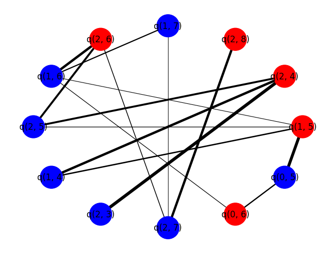
Cut size: 30.930000000000003


-----RANDOM-----
Cut size: 30.030000000000005
For this problem instance, one should see that \(p = 1\) QAOA performs better, on average, than randomly guessing.
